
At the end of April, we released our largest update to go-ipfs to date: IPFS 0.5 (opens new window). While there have been many improvements, the changes to IPFS’s Distributed Hash Table (DHT) were especially critical to improving the performance and stability of finding data in IPFS. For some background on how we arrived at the most recent set of DHT changes, take a look at The Road to the New DHT (opens new window), or try them out yourself in the latest version of go-ipfs (opens new window).
In this post we’d like to take you through the details of what the DHT looks like in v0.5.0, so get ready for a monster post that truly dives deep into the ins and outs of the IPFS DHT implementation. If you want to learn a thing or two about how DHTs work, and how we made the implementation used by IPFS faster and more resilient, read on!
# Background: What does the DHT do for IPFS?
A DHT is a distributed system for mapping keys to values. In IPFS, the DHT is used as the fundamental component of the content routing system. It maps what the user is looking for (a CID) to the peer that is actually storing the matching content. There are 3 types of key-value pairings that are mapped using the DHT:
- Provider Records: These map a data identifier (i.e., a multihash) to a peer that has advertised that they have, and are willing, to provide you with that content.
- Used by IPFS to find content
- Used by IPNS over PubSub to find other members of the pubsub topic
- IPNS Records: These map an IPNS key (i.e., hash of a public key) to an IPNS record (i.e., a signed and versioned pointer to some path like
/ipfs/bafyXYZ)- Used by IPNS
- Peer Records: These map a peerID to a set of multiaddresses at which the peer may be reached
- Used by IPFS when we know of a peer with content, but do not know its address
- Used for manual connections (e.g.,
ipfs swarm connect /p2p/QmXYZ)
Each of these record types has slightly different semantics, but they are all updated and found via the same DHT protocol, IPFS’s take on Kademlia.
# Kademlia Overview
The Kademlia algorithm has been around for a while and there are some great resources already available for it online, including the paper itself (opens new window) and Wikipedia (opens new window). We’ll go through some of the basics here, though.
The general idea of Kademlia is to build a DHT on top of three system parameters:
- An address space: a way that all of the peers in the network can be uniquely identified (in IPFS this is all the numbers from
0to2^256-1) - A metric to order the peers in the address space and therefore visualize all the peers along a line ordered from smallest to largest (in IPFS we we take
SHA256(PeerID)and interpret it as an integer between0and2^256-1) - A projection, that will take a record key and calculate a position in the address space where the peer(s) most ideally suited to store the record should be near (in IPFS we use
SHA256(Record Key))
Having this address space and a peer ordering metric allows us to search the network as though it was a sorted list. In particular, we can turn the system into something like a skip list where a peer knows peers that are distances of around 1,2,4,8,16… away from it. This will allow us to search the list in time that is logarithmic in the size of the network (i.e. O(log(N)) lookup time). Unlike a skip list, Kademlia is somewhat unstable since peers can join, leave and rejoin the network at any time. To deal with the unstable nature of the system, a Kademlia peer does not just keep links to the peers with distance 1,2,4,8,... away from it, but instead for each multiple of 2 away it keeps up to K (in IPFS 20) links. For example, instead of a peer keeping a single link 128 away it would keep 20 links that are between 65 and 128 away.
Note that the selection of network wide parameters like K is not arbitrary, but is instead determined based on the observed average churn in the network and the frequency with which the network will republish information. System parameters (like K) are computed to maximize the probability that the network stays connected and no data is lost, while maintaining a desired latency for queries, and assuming the observations (of average churn) stay constant. These system and network parameters drive the decisions made in Kademlia’s two main components, the routing table which tracks all those links in the network, and the lookup algorithm which determines how to traverse those links to store and retrieve data.
# Kademlia and Undialable Peers
As noted above, a major property of Kademlia is that all peers can be assembled inline from smallest to largest. This property is useful since it means that as peer 0 walks down the line to find peer 55 it can know it is getting progressively closer. However, this requires that everyone on the line can talk to each other, otherwise peer 33 might send peer 0 down a dead end by telling them the content they want is on a node they can’t communicate with. This can result in the network being slow, and more importantly, fragmented with data being accessible by some peers and not others.
While having peers that cannot talk to each other may sound like an oddity, two common causes of peers being unreachable by other peers are NATs and firewalls. For example, having asymmetrical networks where a set of peers X, Y, Z can connect to each other and to A, but A cannot connect to them is fairly common on the modern internet. Similarly, it is extremely common that two peers A and B which are both behind NATs cannot talk to (or dial) each other.
When the IPFS network grew 30x in 2019, we ran into a large problem: suddenly most of the peers on the IPFS DHT were behind NATs, which degraded quality since you couldn’t dial the peer that was supposed to have a given piece of content. To deal with this problem, we now have peers ignore anyone they think is not reachable by the general public, and have peers filter themselves out of the network if they suspect they are not reachable.
To do this, we use libp2p’s AutoNAT, which acts as a distributed STUN layer informing peers of their observed addresses and whether or not they appear to be publicly dialable. Only when peers detect that they are publicly dialable do they switch from client mode (where they can query the DHT, but not respond to queries) to server mode (where they can both query and respond to queries). Similarly, if a server discovers that it is no longer publicly dialable it will switch back into client mode.
Serving AutoNAT requests (i.e., checking whether other peers were dialable) was previously only enabled on opt-in nodes like some of the IPFS public infrastructure. However, leaning so heavily on AutoNAT to clean up undialable nodes from the DHT made us push to make AutoNAT more distributed. Therefore, we now expose a rate-limited AutoNAT service on all IPFS nodes that have discovered that they are publicly dialable. These requests should be infrequent and therefore not have noticeable overhead for standard IPFS nodes.
Note: this automatic switching between DHT client and server modes is the default configuration option, however it is also possible to set your node to only be a “client” if desired. Misconfiguring your network setup while using any option other than “dht” (automatic mode) or “dhtclient” (client-only mode) has the ability to degrade network performance for yourself and everyone else by adding undialable nodes to the network so please exercise care.
While AutoNAT-based mode switching is great, and we are hopeful that it will clear most of the undialable nodes out of the network, it seems only prudent that DHT peers (both clients and servers) should also verify whether nodes appear publicly dialable (e.g., advertise public IP addresses and not just ones like 192.168.X.Y) before either adding them to their routing tables or issuing queries to them.
# Two IPFS DHTs: Public and Local
While many of our users utilize the publicly shared DHT to discover and advertise content, some of them operate in segregated networks (e.g., local networks or isolated VPNs). For these users, having a DHT where all non-publicly dialable nodes are clients is very problematic since NONE of the nodes are publicly dialable.
To make things easier for this use case, we have added a second DHT that is meant to include nodes that are not part of the public network, such as VPNs, CJDNS, Yggdrasil, etc. For now, we’ll refer to this as the LAN DHT, as opposed to the public network which is the WAN DHT. These two DHTs are separated by utilizing different DHT protocol names (i.e., /ipfs/kad/1.0.0 for the WAN DHT, and /ipfs/lan/kad/1.0.0 for the LAN DHT) to eliminate any accidental merging of the two networks. However, all of the non-public networks do have some risk of merging if users have not properly configured their networks.
The main implementation difference between the WAN and LAN DHTs are the acceptance criteria for peers—which are eligible to be part of a routing table or query and which are not. The WAN DHT’s criteria is “do you look like a public address” and the LAN DHT’s criteria is “do you look like a non-public address.” However, while WAN DHT nodes switch from client to server mode based on whether they are publicly dialable, LAN DHT nodes are always servers (unless the “dhtclient” option has been set).
# Routing Tables
As mentioned earlier, every peer in a Kademlia network maintains links to various other peers in the network. The way this works is as follows:
- When we connect to a peer, check if it qualifies to be added to our routing table
- Ensure the peer is a DHT server that is advertising the DHT protocol ID (in IPFS
/ipfs/kad/1.0.0for the public/WAN DHT and/ipfs/lan/kad/1.0.0for the LAN DHT) - Ensure the peer has IP addresses that match the ranges we expect (e.g. members of the public DHT having at least one public range IP address as opposed to only addresses like
192.168.X.Y)
- Ensure the peer is a DHT server that is advertising the DHT protocol ID (in IPFS
- If it qualifies, then determine how close the new peer is in the Kademlia address space to us to figure out which “bucket” it should go into (i.e. if the peer is between 2^7 and 2^8 away from us and the address space is of size 2^256 then the peer goes into bucket 256-8)
- Attempt to put the peer in the bucket
- If the bucket is not full (i.e., has less than 20 peers in it) then add the peer
- If the bucket is full then determine if there are any peers that are "replaceable" (defined below), and then drop one of them and replace it with the new peer. Otherwise, don’t add the peer to the bucket
- If we ever try to query a peer that is in our routing table and fail, then evict them
- Note: After every refresh (see below) we go through the routing table and attempt to connect to peers that we have not queried “recently” to check if they are still online and valid peers for our routing table. If not, then we evict them.
Additionally, in order to keep the routing tables accurate and up to date, we periodically refresh the routing tables. The frequency of the routing table refresh is calculated from a similar set of metrics as the bucket size (you can increase the frequency of refreshes, but there is a floor for how low it may go). For IPFS the floor frequency was selected to be once every 10 minutes. While this is likely a higher frequency than is strictly necessary, we felt it was important to protect the health of the network as we learn more about the IPFS DHT network dynamics post-adoption of go-ipfs v0.5.0.
A routing table refresh works as follows:
- Go through all the buckets, from bucket 0 (the one with peers that are on a different half of the network than we are) up until the highest bucket we have that contains a peer in it (we cap this at bucket 15 due to implementation concerns). For each bucket select a random address in Kademlia space that could fit in that bucket (e.g., in selecting a random peer between 512 and 1024 we selected 678 even though that peer likely does not exist in the network) and do a lookup to find the
Kclosest peers to that random address. This will ensure that we will have filled up each bucket with as many peers as will fit. - We also search for ourselves in the network (i.e., bucket 255), just in case the network size and distribution are such that the first 15 buckets do not suffice for us to learn about the
Kpeers closest to us.
# Lookup Algorithm
The lookup algorithm answers the question “What are the K closest peers to X?”. Our implementation of the Kademlia lookup algorithm goes like this:
- Load the
Kclosest peers toXfrom our routing table into the query queue - Allowing up to Alpha concurrent queries (Alpha in go-ipfs is 10, but is an implementation parameter not inherent in the network itself) grab the peer closest to
Xand ask them “who are theKclosest peers toX?” - When a query to a peer completes add those results to the query queue, and pull the next, closest peer off the queue and query them
- The query terminates whenever the closest known Beta peers to
Xhave been successfully queried (i.e. no dial timeouts, errors, etc.).- Note: Beta is a network wide parameter designed to give some resiliency to the network, it is set to 3 for IPFS.
- After the query is done take the
Kclosest peers that we have not already failed at querying (i.e. we have heard from them or they are still in our queue) and return them- Note: for some API compatibility reasons go-ipfs also ensures that we have actually sent queries to all of the top
Kpeers
- Note: for some API compatibility reasons go-ipfs also ensures that we have actually sent queries to all of the top
In the routing table section, we mentioned that we evict peers that are "replaceable" if we find a new peer that could take their spot in the bucket.
In v0.5.0 we define a peer as "replaceable" if they have not been "useful" to us within the time period during which they are probabilistically expected to have been utilized in a refresh. That value is Log(1/K) * Log(1 - Alpha/K) * refreshPeriod, where Alpha is the number of peers dialed that can be simultaneously queried. Additionally, we define “useful” as responding within 2x the time it takes any other peer from our routing table to respond to us (this biases against peers that are slow, overloaded, unreliable, or have bad network connectivity to us). The definitions of replaceable and useful peers are likely to change as we gather more information about the dynamics of the network and investigate relevant threat models.
# Routing Particulars
While the lookup algorithm is what allows us to put and get records into the DHT, the way in which this is done is slightly different for each record type:
- Provider Records (for a block with Multihash
H)- Put: Do a standard lookup for the
Kclosest peers toSHA256(H)- Put the provider record at those
Kclosest peers (and also store it ourselves) - Note: Currently you are only allowed to put a provider record for yourself (i.e. Alice cannot advertise that Bob has content)
- Put the provider record at those
- Get: Do a lookup for the
Kclosest peers toX=SHA256(H), but instead of just asking each peer in the lookup “who are theKclosest peers toXyou know about?” also ask “please send me the record corresponding toXif you have it”.- The peer adds all new providers it has learned about and continues until the lookup terminates. Depending on which API is used, the lookup can also be forced to abort after receiving a certain number of provider records.
- Put: Do a standard lookup for the
- IPNS Records (For an IPNS key where the multihash of the public key is
H)- Put: Do a standard lookup for the
Kclosest peers toSHA256(../assets/ipns/H)- Put the IPNS record at those
Kclosest peers (and also store it ourselves)
- Put the IPNS record at those
- Get: Do a lookup for the
Kclosest peers toX=SHA256(../assets/ipns/H), but instead of just asking each peer in the lookup “who are theKclosest peers toXyou know about?” also ask “please send me the record corresponding toXif you have it”.- If a user receives a newer record (i.e., a record that has a higher IPNS sequence number), it updates its existing one and continues until the lookup terminates. This is needed in order to make sure that the user gets the latest record. Recall that IPNS records are mutable and therefore, we need to make sure that we point a request to the latest version of the content.
- The default in go-ipfs will abort early after receiving 16 records, but it can be set to go until the query terminates
- Once the lookup is done, if any of the
Kclosest peers toXdid not have the newest IPNS record, send them the newest record
- If a user receives a newer record (i.e., a record that has a higher IPNS sequence number), it updates its existing one and continues until the lookup terminates. This is needed in order to make sure that the user gets the latest record. Recall that IPNS records are mutable and therefore, we need to make sure that we point a request to the latest version of the content.
- Put: Do a standard lookup for the
- Peer Records (For a peer where the multihash of the public key is
H)- Put: This occurs implicitly - when libp2p peers connect to each other they exchange peer information automatically. Being part of the DHT (as either a client or server) requires being in frequent contact with your
Kclosest peers, therefore they will inherently end up with your peer record. - Get: Do a lookup for the
Kclosest peers toX=SHA256(H), but instead of just asking each peer in the lookup “who are theKclosest peers toXyou know about?” also ask “please send me the peer record forHif you have it”- We will try to connect to the peer with ID
Has soon as we learn addresses about it. The lookup can terminate early if we end up connecting to the peer.
- We will try to connect to the peer with ID
- Put: This occurs implicitly - when libp2p peers connect to each other they exchange peer information automatically. Being part of the DHT (as either a client or server) requires being in frequent contact with your
# Testing and Results
There have been a lot of changes to the DHT as part of the go-ipfs v0.5.0 release. While many of the changes were intuitively going to be quite useful, we needed harder evidence that the full set of changes would result in a stable and performant network. To that end, we utilized Testground, which is a new distributed testing infrastructure (check out their launch notes at Testground blog post (opens new window)).
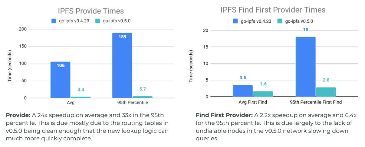
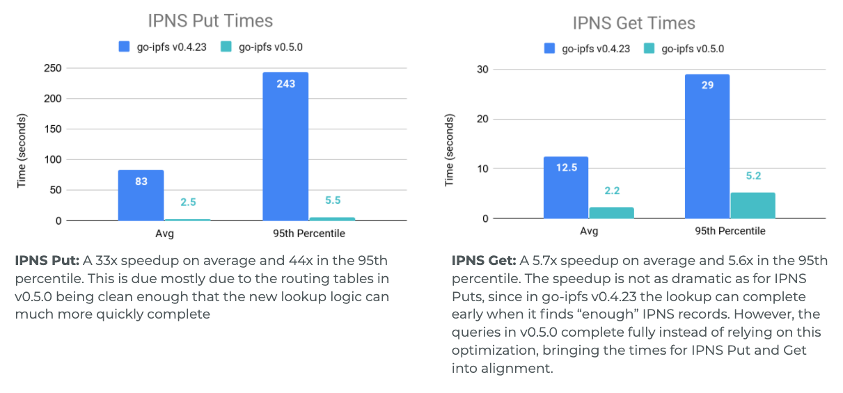
Throughout the development process we ran many Testground tests to get an understanding of how our changes have improved the network. Below is a comparison of the performance of a 1000 peer network where all peers have around 100-120ms latencies from each other, that is running the DHT from go-ipfs v0.4.23 and the DHT from go-ipfs v0.5.0. Note: The v0.4.23 DHT had small modifications to make testing easier like removing hard coded lookup timeouts, so we can see just how long the queries should really be running for.
As can be seen in the graphs, the most drastic changes are to 95th percentile lookup times and to the operations that spent more time doing their lookups and could not terminate as early. This meant IPFS Provide and IPNS Put, which require actually completing a search through the network, got a very large boost (for Provide 24x speedup on average and 33x speedup for the 95th percentile). This was followed by IPNS Get which needs to find many records, then Find Peer which is looking for one very specific record, and finally the time to find just one IPFS Provider record was sped up by 2.2x on average and 6.4x for the 95th percentile.
# Parting Thoughts
Phew! If you have made it all the way through this blog post (or even just skimmed most of it), I commend you! Before sending you back to your exciting lives — just a few brief comments about IPFS v0.5.0 and the releases to come:
IPFS v0.5.0 included a lot of DHT changes and improvements. Something to watch out for is that new nodes are currently participating in the same DHT as older go-ipfs v0.4.23 and earlier nodes. While the DHT code for v0.5.0 is much improved over previous versions, a single node in a big network can only help so much. This means you should see improved performance today when you run v0.5.0, but as more of the network upgrades to v0.5.0 and beyond we will continue to see lookup times improve. So tell your friends it’s time to upgrade! 😁
There are many more exciting improvements to come - so if you are interested in contributing or just tracking our improvements, follow our repositories on GitHub (opens new window) and come chat with us on IRC (opens new window).
# Learn more
- IPFS 0.5.0 Announcement: https://blog.ipfs.tech/2020-04-28-go-ipfs-0-5-0/
- Release Highlights: https://www.youtube.com/watch?v=G8FvB_0HlCE
- Testground: https://blog.ipfs.tech/2020-05-06-launching-testground/